
Matched-Field Processing - Synthetic 2D case
The match-field processing performed in this code is inspired from the one describe in this git repository. The description below is taken from this repository.
The beamformer formulation is written in the frequency domain as:
where \(K_{jk}(\omega) = d_j(\omega) d_k^H(\omega)\) is the cross-spectral density matrix of the recorded signals \(d\), and \(S_{jk}(\omega) = s_j(\omega) s_k^H(\omega)\) is the cross-spectral density matrix of the synthetic signals \(s\).
Here, \(j\) and \(k\) identify sensors, and \(H\) denotes the complex conjugate. Auto-correlations (\(j = k\)) are excluded because they contain no phase information. Consequently, negative beam powers indicate anti-correlation.
The synthetic signals \(s\) (often called replica vectors or Green’s functions) represent the expected wavefield for a given source origin and medium velocity, most often in an acoustic homogeneous half-space \(s_j = \exp(-i \omega t_j)\) where \(t_j\) is the travel time from the source to each receiver \(j\).
The travel time is computed as:
with \(| \mathbf{r}_j - \mathbf{r}_s |\) being the Euclidean distance between the sensor and the source, and \(c\) the medium velocity.
Using this formulation the Bartlett \(B\) in contained in \([-1,1]\).
[ ]:
from itertools import product
import dask.array as da
import matplotlib.pyplot as plt
import numpy as np
import xarray as xr
import pylab as plt
import torch
from tqdm import tqdm

# specific das_ice function
import das_ice.io as di_io
import das_ice.signal.filter as di_filter
import das_ice.processes as di_p
import das_ice.plot as di_plt
import das_ice.mfp as di_mfp

# classic librairy
import torch
import xarray as xr
import pandas as pd
import numpy as np
import matplotlib.pyplot as plt
from matplotlib.colors import LogNorm
%matplotlib inline
[3]:
from dask.distributed import Client,LocalCluster

cluster = LocalCluster(n_workers=8)
client = Client(cluster)
client.dashboard_link
[3]:
'http://127.0.0.1:8787/status'
Defined captor position
In this exemple, 4 sensors are defined.
[4]:
nb_sensor=4
random_sensor=[]
for i in range(nb_sensor):
    random_sensor.append([np.random.randint(-70, 71),np.random.randint(-70, 71),0])

sensors=np.array(random_sensor)
Generate signal
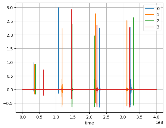
This section shows how to genrate signal that are similar to DAS data. Two events are compute.
[6]:
nb_sources=4
random_sources=[]
for i in range(nb_sources):
    random_sources.append([np.random.randint(-70, 71),np.random.randint(-70, 71),0])
    if i==0:
        dart=di_mfp.artificial_sources_freq(sensors,random_sources[-1],2500,window_length=.1,sampling_rate=25000)
    else:
        dart2=di_mfp.artificial_sources_freq(sensors,random_sources[-1],2500,window_length=.1,sampling_rate=25000)
        dart2['time']=dart2['time']+dart['time'][-1]+dart['time'][1]
        dart=xr.concat([dart,3*dart2],'time')

plt.figure()
for i in range(dart.shape[0]):
    dart[i,:].plot(label=i)

plt.legend()
plt.grid()
[7]:
dart2
[7]:
<xarray.DataArray (distance: 4, time: 2501)> Size: 80kB
array([[-0.00055941,  0.00055953, -0.00055946, ...,  0.00055629,
        -0.00055744,  0.00055748],
       [-0.00092802,  0.00093086, -0.00093362, ...,  0.0009191 ,
        -0.00092211,  0.00092503],
       [-0.00037042,  0.00037006, -0.00037069, ...,  0.00037012,
        -0.0003703 ,  0.00037064],
       [-0.00064768,  0.00064872, -0.00064954, ...,  0.00064358,
        -0.00064489,  0.00064615]], shape=(4, 2501))
Coordinates:
  * time     (time) float64 20kB 3.001e+08 3.002e+08 ... 4.001e+08 4.001e+08
Dimensions without coordinates: distancePerformed MFP
This MPF implementation if taken from the dask implementation from this git repository.
3D MFP
Example of 3D MFP.
[6]:
help(di_mfp.MFP_3D_series)
Help on function MFP_3D_series in module das_ice.mfp:

MFP_3D_series(ds, delta_t, stations, xrange=[-100, 100], yrange=[-100, 100], zrange=[-100, 100], vrange=[2500, 2500], freqrange=[100, 200], dx=5, dy=5, dz=5, dv=250, n_fft=None)
    Perform Matched Field Processing (MFP) on 3D series data to compute beamforming power
    over a range of spatial coordinates, velocities, and frequencies.

    :param ds: Input data as an xarray DataArray containing waveform data.
               Must include 'distance' and 'time' coordinates.
    :type ds: xarray.DataArray

    :param delta_t: Time window size (in seconds) for processing the data in small chunks.
    :type delta_t: float

    :param stations: List of station coordinates used for processing.
    :type stations: list of tuples or ndarray of shape (n_stations, 3)

    :param xrange: Range of horizontal x-coordinates to search (start and end), default is [-100, 100].
    :type xrange: list of float or int

    :param yrange: Range of horizontal y-coordinates to search (start and end), default is [-100, 100].
    :type yrange: list of float or int

    :param zrange: Range of depths to compute (start and end), default is [-100, 100].
    :type zrange: list of float or int

    :param vrange: Velocity range to search in m/s (start and end), default is [2500, 2500].
    :type vrange: list of float or int

    :param freqrange: Frequency range for processing in Hz (start and end), default is [100, 200].
    :type freqrange: list of float

    :param dx: Spacing between grid points in the horizontal x dimension, default is 5.
    :type dx: float or int

    :param dy: Spacing between grid points in the horizontal y dimension, default is 5.
    :type dy: float or int

    :param dz: Spacing between grid points in the depth dimension (z), default is 5.
    :type dz: float or int

    :param dv: Spacing between velocities, default is 250.
    :type dv: float or int

    :return: A 4D xarray DataArray containing the computed beampower values. The dimensions are
             'velocity', 'true_time', 'x', 'y', 'z'.
    :rtype: xarray.DataArray
[14]:
sensors.shape
[14]:
(4, 3)
[8]:
MFP3D=di_mfp.MFP_3D_series(dart,0.1,sensors,xrange=[-70,70],yrange=[-71,71],zrange=[0,0],dx=1,dy=1,dz=1,n_fft=None)
/home/chauvet/miniforge3/envs/taconaz2025/lib/python3.11/site-packages/distributed/client.py:3363: UserWarning: Sending large graph of size 13.55 MiB.
This may cause some slowdown.
Consider loading the data with Dask directly
 or using futures or delayed objects to embed the data into the graph without repetition.
See also https://docs.dask.org/en/stable/best-practices.html#load-data-with-dask for more information.
  warnings.warn(
Filename: /home/chauvet/Documents/Gitlab/das_ice/das_ice/mfp.py

Line #    Mem usage    Increment  Occurrences   Line Contents
=============================================================
   114    778.8 MiB    778.8 MiB           1   @profile
   115                                         def MFP_3D_series(ds,delta_t,stations,xrange=[-100,100],yrange=[-100,100],zrange=[-100,100],vrange=[2500,2500],freqrange=[100,200],dx=5,dy=5,dz=5,dv=250,n_fft=None):
   116                                             '''
   117                                             Perform Matched Field Processing (MFP) on 3D series data to compute beamforming power
   118                                             over a range of spatial coordinates, velocities, and frequencies.
   119
   120                                             :param ds: Input data as an xarray DataArray containing waveform data.
   121                                                        Must include 'distance' and 'time' coordinates.
   122                                             :type ds: xarray.DataArray
   123
   124                                             :param delta_t: Time window size (in seconds) for processing the data in small chunks.
   125                                             :type delta_t: float
   126
   127                                             :param stations: List of station coordinates used for processing.
   128                                             :type stations: list of tuples or ndarray of shape (n_stations, 3)
   129
   130                                             :param xrange: Range of horizontal x-coordinates to search (start and end), default is [-100, 100].
   131                                             :type xrange: list of float or int
   132
   133                                             :param yrange: Range of horizontal y-coordinates to search (start and end), default is [-100, 100].
   134                                             :type yrange: list of float or int
   135
   136                                             :param zrange: Range of depths to compute (start and end), default is [-100, 100].
   137                                             :type zrange: list of float or int
   138
   139                                             :param vrange: Velocity range to search in m/s (start and end), default is [2500, 2500].
   140                                             :type vrange: list of float or int
   141
   142                                             :param freqrange: Frequency range for processing in Hz (start and end), default is [100, 200].
   143                                             :type freqrange: list of float
   144
   145                                             :param dx: Spacing between grid points in the horizontal x dimension, default is 5.
   146                                             :type dx: float or int
   147
   148                                             :param dy: Spacing between grid points in the horizontal y dimension, default is 5.
   149                                             :type dy: float or int
   150
   151                                             :param dz: Spacing between grid points in the depth dimension (z), default is 5.
   152                                             :type dz: float or int
   153
   154                                             :param dv: Spacing between velocities, default is 250.
   155                                             :type dv: float or int
   156
   157                                             :param n_fft: n in torch.fft.fft function
   158                                             :type dv: int
   159
   160                                             :return: A 4D xarray DataArray containing the computed beampower values. The dimensions are
   161                                                      'velocity', 'true_time', 'x', 'y', 'z'.
   162                                             :rtype: xarray.DataArray
   163                                             '''
   164
   165    778.9 MiB      0.0 MiB           1       sampling_rate=(ds.time[1]-ds.time[0]).values.astype(float)*10**-9
   166                                             # defined number of sample per time series
   167    778.9 MiB      0.0 MiB           1       dn=int(delta_t/sampling_rate)
   168                                             # build a data cube with a dimention for each time series
   169    778.9 MiB      0.0 MiB           1       ll=[]
   170    778.9 MiB      0.0 MiB           1       true_time=[]
   171    778.9 MiB      0.0 MiB           1       din=int(len(ds.time)/dn)
   172    778.9 MiB      0.0 MiB           5       for i in range(din):
   173    778.9 MiB      0.0 MiB           4           tmp=ds[:,i*dn:(i+1)*dn]
   174    778.9 MiB      0.0 MiB           4           new_time = np.arange(dn) * sampling_rate
   175    778.9 MiB      0.0 MiB           4           true_time.append(tmp.time[0].values)
   176    778.9 MiB      0.0 MiB           4           tmp = tmp.assign_coords(time=new_time)
   177    778.9 MiB      0.0 MiB           4           ll.append(tmp)
   178    778.9 MiB      0.0 MiB           1       ds_cube=xr.concat(ll,dim='true_time')
   179                                             ############
   180                                             ##
   181                                             ############
   182    778.9 MiB      0.0 MiB           1       if n_fft is None:
   183    778.9 MiB      0.0 MiB           1           n_fft=len(ds_cube.time)
   184                                             else:
   185                                                 sampling_rate*=len(ds_cube.time)/n_fft
   186
   187
   188                                             # Fiber signal processing
   189    779.8 MiB      0.9 MiB           1       multi_waveform_spectra=torch.fft.fft(torch.from_numpy(ds_cube.values),axis=2,n=n_fft).to(dtype=torch.complex128)
   190    779.8 MiB      0.0 MiB           1       freqs = torch.fft.fftfreq(n_fft,sampling_rate)
   191                                             # Normalized over each frequencies
   192    780.4 MiB      0.5 MiB           1       spectral_norm = torch.abs(multi_waveform_spectra) # Spectral norm
   193                                             # Replace 0 values with 1
   194    781.3 MiB      0.9 MiB           1       spectral_norm[spectral_norm == 0] = 1
   195    781.9 MiB      0.7 MiB           1       multi_waveform_spectra = multi_waveform_spectra/spectral_norm
   196                                             #
   197    781.9 MiB      0.0 MiB           1       omega = 2 * torch.pi * freqs
   198                                             # frequency sampling
   199    782.2 MiB      0.3 MiB           1       freq_idx = torch.where((freqs >= freqrange[0]) & (freqs <= freqrange[1]))[0]
   200    782.3 MiB      0.1 MiB           1       omega_lim = omega[freq_idx]
   201    782.4 MiB      0.1 MiB           1       waveform_spectra_lim = multi_waveform_spectra[:,:,freq_idx]
   202
   203
   204
   205    782.6 MiB      0.2 MiB           1       K = waveform_spectra_lim[:,:, None, :] * waveform_spectra_lim.conj()[:,None, :, :]
   206    782.6 MiB      0.1 MiB           1       diag_idxs = torch.arange(K.shape[1])
   207    782.8 MiB      0.2 MiB           1       zero_spectra = torch.zeros(omega_lim.shape, dtype=torch.cdouble)
   208    782.9 MiB      0.1 MiB           1       K[:,diag_idxs, diag_idxs, :] = zero_spectra
   209    782.9 MiB      0.0 MiB           1       K = da.from_array(K.numpy())
   210
   211                                             # Compute grid
   212    782.9 MiB      0.0 MiB           1       x_coords = torch.arange(xrange[0], xrange[1] + dx, dx)
   213    782.9 MiB      0.0 MiB           1       y_coords = torch.arange(yrange[0], yrange[1] + dy, dy)
   214    782.9 MiB      0.0 MiB           1       z_coords = torch.arange(zrange[0], zrange[1] + dz, dz)
   215    782.9 MiB      0.0 MiB           1       v_coords=torch.arange(vrange[0], vrange[1] + dv, dv)
   216    783.8 MiB      0.8 MiB           1       gridpoints = torch.tensor(list(product(x_coords, y_coords, z_coords)))
   217
   218    783.8 MiB      0.0 MiB           1       stations=torch.tensor(stations).to(dtype=torch.complex128)
   219    783.8 MiB      0.1 MiB           1       distances_to_all_gridpoints = torch.linalg.norm(gridpoints[:, None, :] - stations[None, :, :], axis=2)
   220
   221                                             # Compute traveltimes
   222    783.8 MiB      0.0 MiB           1       traveltimes=distances_to_all_gridpoints[None,:,:]/v_coords[:,None,None]
   223    797.4 MiB     13.5 MiB           1       greens_functions = torch.exp(-1j * omega_lim[None, None,None, :] * traveltimes[:, :, :, None])
   224                                             # move critical part to dask
   225    810.9 MiB     13.5 MiB           1       greens_functions_dask = da.from_array(greens_functions.numpy(), chunks='auto')
   226    810.9 MiB      0.0 MiB           1       S = (greens_functions_dask[:, :,:, None,:]*greens_functions_dask.conj()[:,:, None, :,:])
   227                                             # Perform the einsum operation
   228    810.9 MiB      0.0 MiB           1       beampowers_d = da.einsum("vlgijw, ljiw -> vlg", S[:, None , :, :, :, :], K).real
   229    824.5 MiB     13.6 MiB           1       beampowers = beampowers_d.compute()
   230    824.5 MiB      0.0 MiB           1       bp = beampowers.reshape(len(v_coords),din, len(x_coords), len(y_coords), len(z_coords))
   231
   232    824.5 MiB      0.0 MiB           1       res=xr.DataArray(bp,dims=['velocity','true_time','x','y','z'])
   233    824.5 MiB      0.0 MiB           1       res['velocity']=v_coords
   234    824.5 MiB      0.0 MiB           1       res['true_time']=true_time
   235    824.5 MiB      0.0 MiB           1       res['x']=x_coords
   236    824.5 MiB      0.0 MiB           1       res['y']=y_coords
   237    824.5 MiB      0.0 MiB           1       res['z']=z_coords
   238
   239    824.5 MiB      0.0 MiB           1       res=res.transpose("x","y","z","velocity","true_time")/((stations.shape[0]-1)*stations.shape[0]*len(omega_lim))
   240
   241    824.5 MiB      0.0 MiB           1       return res
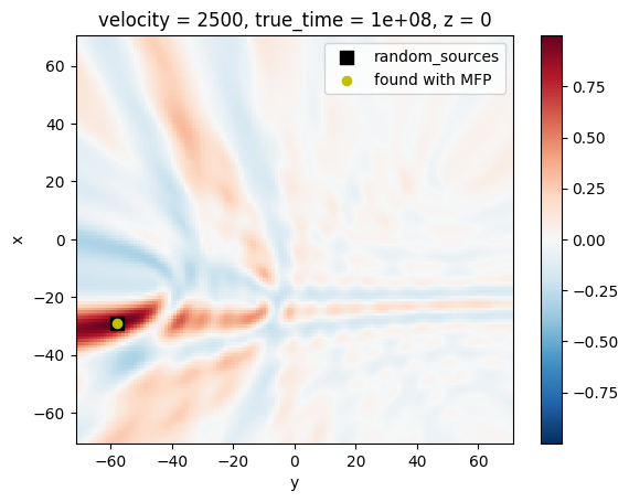
Show results
The MFP is finding the best match for:
[13]:
i_event=1
find_sources=MFP3D[...,i_event].where(MFP3D[...,i_event] == MFP3D[...,i_event].max(), drop=True).coords
find_sources
[13]:
Coordinates:
  * velocity   (velocity) int64 8B 2500
    true_time  float64 8B 1e+08
  * x          (x) int64 8B -29
  * y          (y) int64 8B -58
  * z          (z) int64 8B 0
The true sources was in:
[14]:
matching_index = np.where(MFP3D.z.values == find_sources['z'].values)[0]
MFP3D[...,matching_index,0,i_event].plot()
plt.scatter(random_sources[i_event][1],random_sources[i_event][0],s=80,marker='s',color='k',label='random_sources')
plt.scatter(find_sources['y'],find_sources['x'],s=35,color='y',label='found with MFP')
plt.legend()
[14]:
<matplotlib.legend.Legend at 0x7709f8160610>
3D plot of the MFP Bartlett with a slider to plot the different plane of the Bartlett field.