Quick start
This quick start present data processing using Terra15 DAS recording velocity. It can easily adapted for Febus DAS recording strain rate.
The processing is taking advantage of dask+xarray framework.
[1]:
# specific das_ice function
import das_ice.io as di_io
import das_ice.signal.filter as di_filter
import das_ice.processes as di_p
import das_ice.plot as di_plt

# classic librairy
import xarray as xr
import pandas as pd
import numpy as np
import matplotlib.pyplot as plt
from matplotlib.colors import LogNorm
from tqdm import trange
%matplotlib inline
[2]:
from dask.distributed import Client,LocalCluster

cluster = LocalCluster(n_workers=8)
client = Client(cluster)
client.dashboard_link
[2]:
'http://127.0.0.1:8787/status'
Loading data
[3]:
ds=xr.Dataset()
ds['velocity']=di_io.dask_Terra15('*.hdf5', chunks="auto")
The program reads HDF5 files without loading them entirely into memory. This allows for efficient selection of time and distance ranges before processing. One benefit of using Dask is its ability to handle large datasets that cannot fit into memory. Additionally, Dask enables distributed parallel computing, ensuring efficient execution across multiple processors or machines.
[4]:
ds.velocity
[4]:
<xarray.DataArray 'velocity' (time: 1236726, distance: 618)> Size: 3GB
dask.array<concatenate, shape=(1236726, 618), dtype=float32, chunksize=(54100, 618), chunktype=numpy.ndarray>
Coordinates:
  * distance  (distance) float64 5kB 674.6 678.7 682.8 ... 3.19e+03 3.194e+03
  * time      (time) datetime64[ns] 10MB 2024-08-29T05:04:48.597790 ... 2024-...
Attributes:
    client_fn_applied:
    dT:                  0.000147915811144255
    dx:                  4.083809535485629
    frame_shape:         [1082  618]
    nT:                  1082
    nx:                  618
    recorder_id:         T311542
trigger_start_time: -1.0Data selection
The data used here are from a BoreHole where the optic fiber is doing a loop. Therefore, the depth of the borehole and the bottom of the borehole are used to select the distance range.
[5]:
d_optic_bottom=2505 #m
depth_bh=97 #m
[6]:
ds=ds.sel(distance=slice(d_optic_bottom-depth_bh,d_optic_bottom+depth_bh)).sel(time=slice('2024-08-29T05:05:30','2024-08-29T05:06:30'))
This is a trick to put distance not in optic distance reference frame but in the borehole reference frame.
[7]:
ds['distance']=-1*(np.abs(ds.distance-d_optic_bottom)-depth_bh)
ds = ds.sortby('distance')
Data Filtering
The DAS data were aquired at a sampling frequency higher than \(6000~Hz\).
[8]:
print('sampling frequency: '+str(1/((ds.time[1]-ds.time[0]).values.astype(float)*10**-9))+' Hz')
sampling frequency: 6760.593850563833 Hz
It is posible to decimate the data around \(1000~Hz\). By taking 1 value over 6.
[9]:
dvel_decimated=di_filter.decimate(ds.velocity,6)
[10]:
dvel_decimated
[10]:
<xarray.DataArray 'velocity' (time: 68733, distance: 47)> Size: 13MB
dask.array<getitem, shape=(68733, 47), dtype=float32, chunksize=(9017, 47), chunktype=numpy.ndarray>
Coordinates:
  * distance  (distance) float64 376B 2.264 3.88 6.348 ... 92.11 93.72 96.19
  * time      (time) datetime64[ns] 550kB 2024-08-29T05:05:30.000017080 ... 2...
Attributes:
    client_fn_applied:
    dT:                  0.000147915811144255
    dx:                  4.083809535485629
    frame_shape:         [1082  618]
    nT:                  1082
    nx:                  618
    recorder_id:         T311542
trigger_start_time: -1.0[11]:
print('decimated frequency: '+str(1/((dvel_decimated.time[1]-dvel_decimated.time[0]).values.astype(float)*10**-9))+' Hz')
decimated frequency: 1126.7669113628808 Hz
From velocity to strain rate
Using Terra15 DAS, you might need to convert velocity to strain rate.
[12]:
dsr=di_p.strain_rate(dvel_decimated)
Bandpass filter
If you want to look at the fequency between \(100~Hz\) and \(200~Hz\), you can apply a bandpass filter.
[13]:
dsrf=di_filter.bandpass(dsr,100,200)
Up to here nothing as been process. Dask just build computation tree but no data was loaded.
[14]:
dsrf
[14]:
<xarray.DataArray 'velocity' (time: 68733, distance: 47)> Size: 13MB
dask.array<transpose, shape=(68733, 47), dtype=float32, chunksize=(68733, 47), chunktype=numpy.ndarray>
Coordinates:
  * distance  (distance) float64 376B 2.264 3.88 6.348 ... 92.11 93.72 96.19
  * time      (time) datetime64[ns] 550kB 2024-08-29T05:05:30.000017080 ... 2...
Data Visualisation
Trace with depth
[15]:
dsrf
[15]:
<xarray.DataArray 'velocity' (time: 68733, distance: 47)> Size: 13MB
dask.array<transpose, shape=(68733, 47), dtype=float32, chunksize=(68733, 47), chunktype=numpy.ndarray>
Coordinates:
  * distance  (distance) float64 376B 2.264 3.88 6.348 ... 92.11 93.72 96.19
  * time      (time) datetime64[ns] 550kB 2024-08-29T05:05:30.000017080 ... 2...
[16]:
fig=di_plt.all_trace(dsrf.sel(distance=slice(20,50)))

start_date = pd.to_datetime('2024-08-29T05:06:01.20')
end_date = pd.to_datetime('2024-08-29T05:06:01.70')

# Update the x-axis range
fig.update_xaxes(range=[start_date, end_date])
fig.show("png")

Standard deviation waterfall
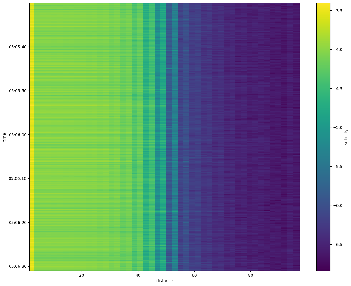
This figure show the standard deviation of the strain rate signal over a time windows of \(\sim 0.2~s\).
[17]:
plt.figure(figsize=(15,12))
dsrfl=dsrf.load()
np.log10(di_p.std_local(dsrfl,nt=200,nx=1))[5:,:].plot()
plt.gca().invert_yaxis()
