Matched-Field Processing - Synthetic 3D case

from itertools import product
import dask.array as da
import matplotlib.pyplot as plt
import numpy as np
import xarray as xr
import pylab as plt
import torch
from tqdm import tqdm
from scipy.signal import ricker

# specific das_ice function
import das_ice.io as di_io
import das_ice.signal.filter as di_filter
import das_ice.processes as di_p
import das_ice.plot as di_plt
import das_ice.mfp as di_mfp

# classic librairy
import torch
import xarray as xr
import pandas as pd
import numpy as np
import matplotlib.pyplot as plt
from matplotlib.colors import LogNorm
from tqdm import trange
%matplotlib inline

from dask.distributed import Client,LocalCluster

cluster = LocalCluster(n_workers=8)
client = Client(cluster)
client.dashboard_link

'http://127.0.0.1:8787/status'

Defined captor position

In this exemple, 4 sensors are defined.

nb_sensor=4
random_sensor=[]
for i in range(nb_sensor):
    random_sensor.append([np.random.randint(-70, 71),np.random.randint(-70, 71),np.random.randint(-70, 71)])

sensors=np.array(random_sensor)

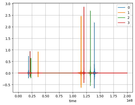
Generate signal

This section shows how to genrate signal that are similar to DAS data. Two events are compute.

nb_sources=2
random_sources=[]
for i in range(nb_sources):
    random_sources.append([np.random.randint(-70, 71),np.random.randint(-70, 71),np.random.randint(-70, 71)])
    if i==0:
        dart=di_mfp.artificial_sources_freq(sensors,random_sources[-1],2500,window_length=.1,sampling_rate=25000)
    else:
        dart2=di_mfp.artificial_sources_freq(sensors,random_sources[-1],2500,window_length=.1,sampling_rate=25000)
        dart2['time']=dart2['time']+dart['time'][-1]+dart['time'][1]
        dart=xr.concat([dart,3*dart2],'time')

plt.figure()
for i in range(dart.shape[0]):
    dart[i,:].plot(label=i)

plt.legend()
plt.grid()

dart2

<xarray.DataArray (distance: 4, time: 2501)> Size: 80kB
array([[-3.84845233e-04,  3.84559707e-04, -3.82843937e-04, ...,
         3.84511713e-04, -3.83519218e-04,  3.83916897e-04],
       [ 3.17374089e-04, -3.17177081e-04,  3.16904569e-04, ...,
        -3.15647239e-04,  3.15769046e-04, -3.16133125e-04],
       [ 4.35114207e-05, -4.53521546e-05,  4.48563355e-05, ...,
        -4.59801400e-05,  4.68964603e-05, -4.60621167e-05],
       [ 4.65646802e-04, -4.66269629e-04,  4.66813232e-04, ...,
        -4.65439188e-04,  4.65992133e-04, -4.65982676e-04]])
Coordinates:
  * time     (time) float64 20kB 1e+08 1.001e+08 1.001e+08 ... 2e+08 2e+08 2e+08
Dimensions without coordinates: distance

xarray.DataArray

• distance: 4
• time: 2501

• -0.0003848 0.0003846 -0.0003828 ... -0.0004654 0.000466 -0.000466

  array([[-3.84845233e-04,  3.84559707e-04, -3.82843937e-04, ...,
           3.84511713e-04, -3.83519218e-04,  3.83916897e-04],
         [ 3.17374089e-04, -3.17177081e-04,  3.16904569e-04, ...,
          -3.15647239e-04,  3.15769046e-04, -3.16133125e-04],
         [ 4.35114207e-05, -4.53521546e-05,  4.48563355e-05, ...,
          -4.59801400e-05,  4.68964603e-05, -4.60621167e-05],
         [ 4.65646802e-04, -4.66269629e-04,  4.66813232e-04, ...,
          -4.65439188e-04,  4.65992133e-04, -4.65982676e-04]])

• Coordinates: (1)
  • time
    (time)
    float64
    1e+08 1.001e+08 ... 2e+08 2e+08

    array([1.0004e+08, 1.0008e+08, 1.0012e+08, ..., 1.9996e+08, 2.0000e+08,
           2.0004e+08])

• Indexes: (1)
  • time
    PandasIndex

    PandasIndex(Index([100040000.0, 100080000.0, 100120000.0, 100160000.0, 100200000.0,
           100240000.0, 100280000.0, 100320000.0, 100360000.0, 100400000.0,
           ...
           199680000.0, 199720000.0, 199760000.0, 199800000.0, 199840000.0,
           199880000.0, 199920000.0, 199960000.0, 200000000.0, 200040000.0],
          dtype='float64', name='time', length=2501))

• Attributes: (0)

Performed MFP

This MPF implementation if taken from the dask implementation from this git repository.

3D MFP

Example of 3D MFP.

help(di_mfp.MFP_3D_series)

Help on function MFP_3D_series in module das_ice.mfp:

MFP_3D_series(ds, delta_t, stations, xrange=[-100, 100], yrange=[-100, 100], zrange=[-100, 100], vrange=[2500, 2500], freqrange=[100, 200], dx=5, dy=5, dz=5, dv=250, n_fft=None)
    Perform Matched Field Processing (MFP) on 3D series data to compute beamforming power
    over a range of spatial coordinates, velocities, and frequencies.

    :param ds: Input data as an xarray DataArray containing waveform data.
               Must include 'distance' and 'time' coordinates.
    :type ds: xarray.DataArray

    :param delta_t: Time window size (in seconds) for processing the data in small chunks.
    :type delta_t: float

    :param stations: List of station coordinates used for processing.
    :type stations: list of tuples or ndarray of shape (n_stations, 3)

    :param xrange: Range of horizontal x-coordinates to search (start and end), default is [-100, 100].
    :type xrange: list of float or int

    :param yrange: Range of horizontal y-coordinates to search (start and end), default is [-100, 100].
    :type yrange: list of float or int

    :param zrange: Range of depths to compute (start and end), default is [-100, 100].
    :type zrange: list of float or int

    :param vrange: Velocity range to search in m/s (start and end), default is [2500, 2500].
    :type vrange: list of float or int

    :param freqrange: Frequency range for processing in Hz (start and end), default is [100, 200].
    :type freqrange: list of float

    :param dx: Spacing between grid points in the horizontal x dimension, default is 5.
    :type dx: float or int

    :param dy: Spacing between grid points in the horizontal y dimension, default is 5.
    :type dy: float or int

    :param dz: Spacing between grid points in the depth dimension (z), default is 5.
    :type dz: float or int

    :param dv: Spacing between velocities, default is 250.
    :type dv: float or int

    :return: A 4D xarray DataArray containing the computed beampower values. The dimensions are
             'velocity', 'true_time', 'x', 'y', 'z'.
    :rtype: xarray.DataArray

sensors.shape

(4, 3)

MFP3D=di_mfp.MFP_3D_series(dart,0.1,sensors,xrange=[-70,70],yrange=[-71,71],zrange=[-72,72],dx=1,dy=1,dz=1,n_fft=5000)

/home/chauvet/miniforge3/envs/das_ice/lib/python3.11/site-packages/distributed/client.py:3362: UserWarning: Sending large graph of size 3.31 GiB.
This may cause some slowdown.
Consider loading the data with Dask directly
 or using futures or delayed objects to embed the data into the graph without repetition.
See also https://docs.dask.org/en/stable/best-practices.html#load-data-with-dask for more information.
  warnings.warn(

Show results

The MFP is finding the best match for:

i_event=0
find_sources=MFP3D[...,i_event].where(MFP3D[...,i_event] == MFP3D[...,i_event].max(), drop=True).coords
find_sources

Coordinates:
  * velocity   (velocity) int64 8B 2500
    true_time  float64 8B 0.0
  * x          (x) int64 8B -27
  * y          (y) int64 8B 6
  * z          (z) int64 8B 17

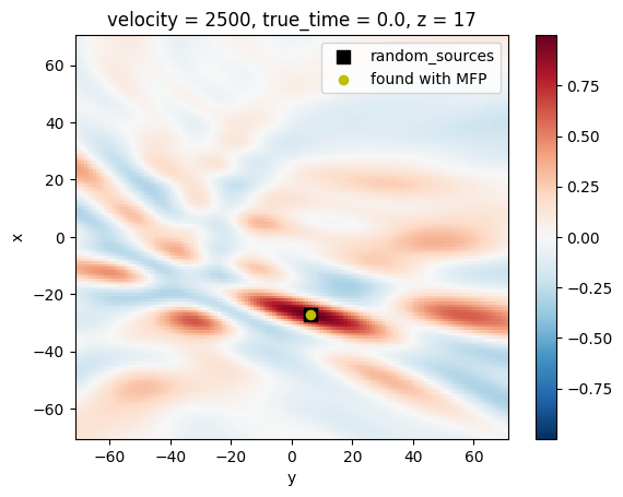
The true sources was in:

random_sources[i_event]

[-27, 6, 17]

matching_index = np.where(MFP3D.z.values == find_sources['z'].values)[0]
MFP3D[...,matching_index,0,i_event].plot()
plt.scatter(random_sources[i_event][1],random_sources[i_event][0],s=80,marker='s',color='k',label='random_sources')
plt.scatter(find_sources['y'],find_sources['x'],s=35,color='y',label='found with MFP')
plt.legend()

<matplotlib.legend.Legend at 0x75e0dc2b4650>

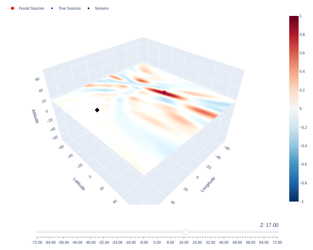
3D plot of the MFP Bartlett with a slider to plot the different plane of the Bartlett field.

fig=di_mfp.plot_MFP3D(MFP3D[...,0,i_event],sensors,true_source=random_sources[i_event])
fig.update_layout(
    scene_camera=dict(
        eye=dict(x=1.2, y=1.2, z=1.2)
    )
)
fig.show("png")